Interactive Maps with tmap and Shiny

Session 1: Introduction to tmap

Martijn Tennekes

Introduction to tmap

Goal

Visualize spatial data
Intuitive to use
Flexible

Software to visualize spatial data

Traditional GIS software: ArcGIS, QGIS, GRASS
Data science programming languages: Python, R, Julia
Web technologies: JavaScript

Traditional GIS software

Proprietary: ArcGIS
Free/open-source: QGIS, GRASS

No programming required
Many options and tools can be difficult to navigate
Workflows often not easily reproducible or scriptable

Data science program languages

Python, R, Julia

Require programming skills
Support scripted, reproducible workflows
Multiple ‘competing’ and complementary packages foster innovation
Large and active communities

R packages

Package	Also non-spatial	Static	Interactive	Extendable
ggplot	✅	✅	-	✅
tmap	-	✅	✅	✅
mapsf	-	✅	-	-
mapview	-	—	✅	-
leaflet	-	—	✅	-
mapgl	-	—	✅	-

tmap and other packages

Compared

Uses

leaflet in its interactive "view" mode
mapgl in its other interactive modes "mapbox" and "maplibre" via tmap.mapgl

JavaScript

Interactive mapping: d3, leaflet, Mapbox GL JS, MapLibre GL JS, etc.
Many R and Python libraries use them under the hood
More flexible to use them directly, but requires significantly more development effort and technical knowledge.

When to Use tmap

✅ Great choice if you want to:

Make publication-quality static maps
Quickly switch to interactive maps for exploration
Use a layered syntax similar to ggplot2
Teach spatial visualization in a clear and structured way
Export maps for reports, articles, or dashboards

🚫 Not ideal for:

Fully customized HTML map apps (use JavaScript directly)
Real-time data interaction or streaming
Very large datasets (consider performance tuning or alternatives)

A brief history of tmap

Evolution

Version	Year	Key changes
0.6	2014	First CRAN release
1.0	2014	Common map layers and components
1.4	2015	Interactive mapping (Leaflet)
2.0	2018	Migration from sp to sf; basemaps
2.3	2019	Shiny integration
3.0	2020	Migration from raster to stars
4.0	2025	Fully extensible; generic layer functions
4.1	2025	Sharper basemaps in plot mode; animation support
4.2	2025	Inset maps and minimap for plot mode
4.3	2026	External data source support; text enhancements
4.4	2026	Layer blending; hitbox for interactive layers

GitHub community (Figure 1)

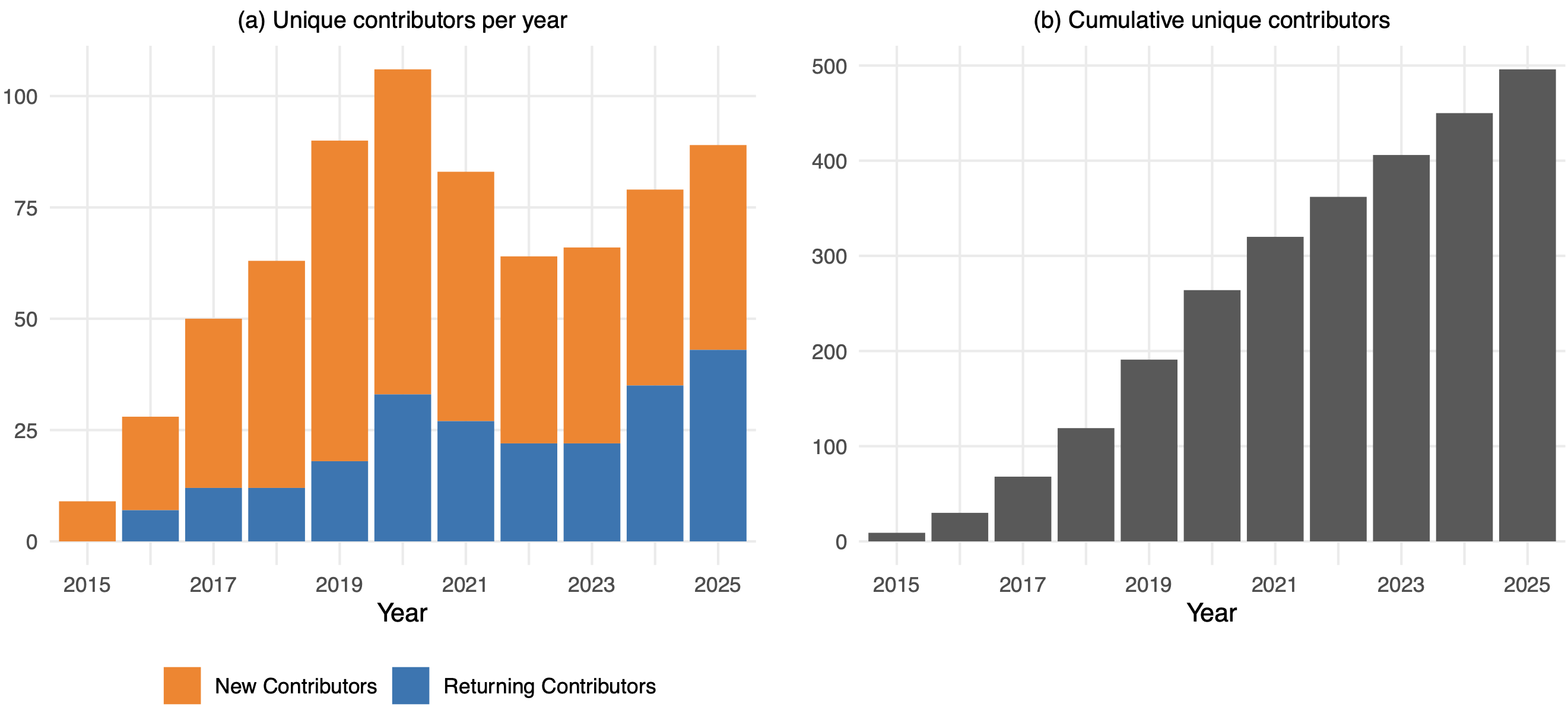
GitHub contributors per year (new and returning). Community growth reflects ongoing adoption and active maintenance since 2014.

What’s new in version 4?

Three core goals of the version 4 rewrite:

Spatial data classes — native support for sf, stars, and terra; extensible to any class
Map layer functions — generic and extendable; consistent syntax for all map variables
Visualization platforms — support for additional rendering modes beyond "plot" and "view"

Extensions (as of 2026)

Package	What it adds
`tmap.cartogram`	`tm_cartogram()` — distorted polygon maps
`tmap.glyphs`	`tm_donuts()`, `tm_flower()` — glyph maps
`tmap.networks`	`tm_edges()`, `tm_nodes()` — network maps
`tmap.mapgl`	`"mapbox"` and `"maplibre"` rendering modes
`tmap.sources`	access remote sources (PMTiles)

All five are on CRAN. Three are in early development; tmap.cartogram is the most mature.

tmap downloads in context (Figure 2)

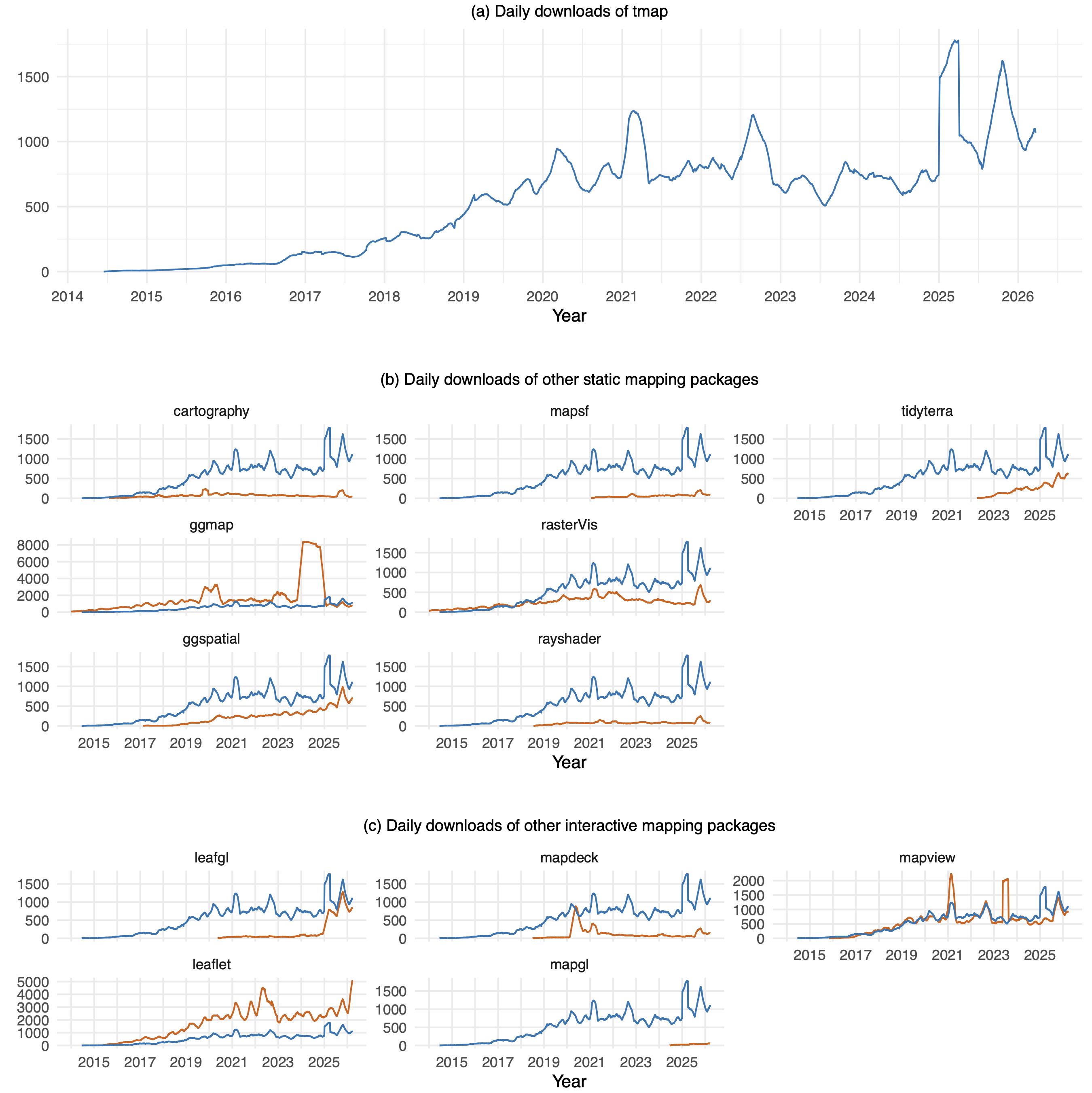
Daily downloads, smoothed 91-day rolling average. Orange = other packages; blue = tmap for comparison. tmap and mapview have remained similarly popular since ~2016.

Grammar of thematic maps

Layered Grammar of Thematic Maps — LGoTM (Figure 3)

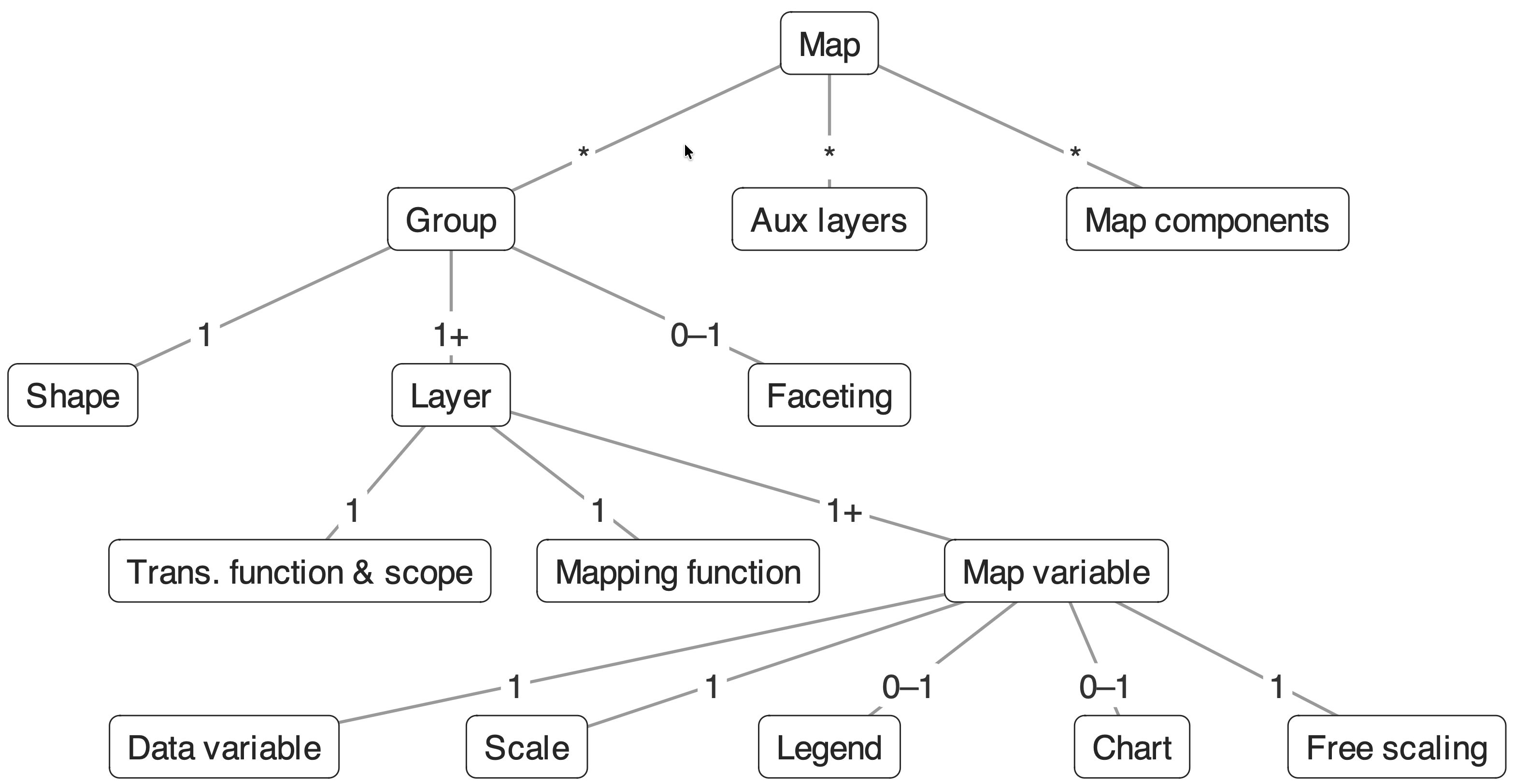
Hierarchical structure of the LGoTM. A Map contains Groups, Aux layers, and Map components. Each Group has a Shape and one or more Layers.

LGoTM in words

A map is composed of groups, each with a shape and one or more layers
Each layer has a transformation function that transforms features before mapping
- Geometric: e.g. tm_dots() applied to polygons → centroids
- Data-driven: e.g. cartograms distort polygon geometry proportional to a variable
Each layer has a mapping function that maps data to visual properties
Map variables (fill, col, size, lwd…) can be constant or data-driven
Each data-driven variable has a scale and optional legend
Auxiliary layers (basemaps, graticules) and map components (scalebar, compass) complete the map

Building blocks in code

tm_shape(NLD_muni) +            # Shape (group 1)
  tm_polygons(                  # Layer: data-driven fill
    fill = "income_high",
    fill.scale = tm_scale_continuous(values = "brewer.purples"),
    fill.legend = tm_legend(title = "Income")) +
tm_shape(NLD_prov) +            # Shape (group 2)
  tm_borders(col = "black", lwd = 2) +
  tm_text(text = "name") +
tm_basemap("Esri.WorldTerrain") +    # auxiliary layer
tm_compass() +                       # map component
tm_scalebar()

LGoTM in practice — NLD choropleth (Figure 4)

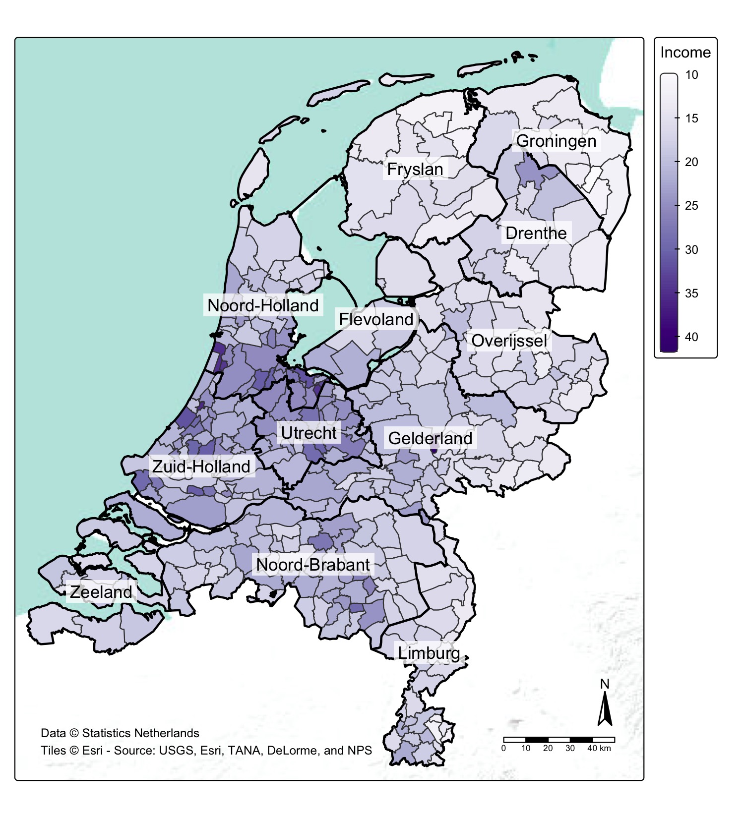
The map above is generated by the code on the previous slide. See tmap4_manuscript_figures.R. It contains two Groups, one auxiliary layer (basemap), and two map components (compass, scalebar).

Naming conventions

tm_ prefix → stackable layer and component functions
tmap_ prefix → standalone utility functions (tmap_mode(), tmap_save() …)
Map variable arguments follow a consistent dot notation:
- fill, fill.scale, fill.legend, fill.chart, fill.free
- Same pattern for col, size, lwd, lty, shape …

Map variables per layer

Layer	Map variables
`tm_polygons`	`fill`, `fill_alpha`, `col`, `col_alpha`, `lwd`, `lty`
`tm_symbols`	`size`, `shape`, `fill`, `fill_alpha`, `col`, `col_alpha`, `lwd`
`tm_lines`	`col`, `col_alpha`, `lwd`, `lty`
`tm_raster`	`col`, `col_alpha`
`tm_text`	`text`, `size`, `col`, `col_alpha`, `fontface`

Each can be constant or data-driven. If data-driven, add .scale and optionally .legend.

Scale functions

Function	Primary use
`tm_scale_continuous()`	colour gradients, symbol size, line width
`tm_scale_intervals()`	classified choropleth (n, style, breaks)
`tm_scale_categorical()`	categorical colour or symbol shape
`tm_scale_rgb()`	RGB raster images
`tm_scale_asis()`	pre-encoded values (e.g. colour column)

Getting started

Step 1: Installation

Instructions

install.packages("tmap")
# or for development version:
remotes::install_github("r-tmap/tmap")

Current CRAN version: 4.3

Step 2: Find demo datasets

Included in tmap:

Vector: World, NLD_prov, NLD_muni, NLD_dist, metro, World_rivers

Raster: land

Other datasets in spData. Large datasets (Zion NP rasters, etc.) in spDataLarge.

Step 3: Your first map

library(tmap)

tm_shape(World) +
  tm_polygons(fill = "HPI")

Switch to interactive with one call:

ttm()   # toggle to "view" mode

tm_shape(World) +
  tm_polygons(fill = "HPI",
              hover = "name",
              popup.vars = c("name", "HPI", "life_exp"))

Step 4: Learn more

Online vignettes — full reference with examples
Geocomputation with R — practical mapping chapter
Spatial Data Visualization with tmap — upcoming book A Practical Guide to Thematic Mapping in R

Recap

tmap is a powerful and flexible R package for spatial data visualization
Version 4 (2025–2026): extensible, generic layer functions, consistent syntax
The same tmap code runs in both static ("plot") and interactive ("view") mode
Extensions add new modes, layer types, and spatial object support
Main documentation