library(tmap)
library(tmap.mapgl)

tmap_mode("maplibre")

tm_shape(World) +
  tm_polygons_3d(
    height = "pop_est_dens",  # variable controlling extrusion height
    fill = "continent"        # variable controlling fill colour
)Interactive Maps with tmap and Shiny
Session 8: 3D maps and high-performance web maps
Martijn Tennekes
3D polygon maps
The tm_polygons_3d() layer
tmap.mapgl introduces a new layer type available only in "mapbox" and "maplibre" modes:
tm_polygons_3d() is identical to tm_polygons() with one additional visual variable: height.
Camera controls: pitch
Use tm_maplibre() to tilt the camera:
In the browser: right-click + drag to tilt interactively.
Example: NLD population density
Height = population density, colour = education level:
tmap_mode("maplibre")

NLD_dist$pop_dens <- NLD_dist$population / NLD_dist$area

tm_shape(NLD_dist) +
  tm_polygons_3d(
    height = "pop_dens",
    fill = "edu_appl_sci",
    fill.scale = tm_scale_intervals(style = "kmeans", values = "-pu_gn"),
    fill.legend = tm_legend("Applied sci. degree (%)"),
    hover = "name"
  ) +
tm_crs(crs = 3857) +
tm_maplibre(pitch = 45)
Interpreting 3D maps
- Height encodes magnitude (e.g. density, count, value)
- Volume therefore represents total (height × area ≈ total count)
- Colour encodes a second variable simultaneously
- Use
pitcharound 30–50° for a good balance of readability and 3D effect - Suitable for urban/administrative data — beware of artefacts in sparse regions
Example: global population (WorldPop 2025)
Data: WorldPop 2025
WorldPop provides global gridded population counts at ~1 km resolution.
- Source: hub.worldpop.org
- File:
global_pop_2025_CN_1km_R2025A_UA_v1.tif - Aggregated by factor 64 to ~59 km × 59 km cells for performance
Aggregating with terra
fact = 64→ 64 × 64 = 4096 cells merged into onefun = sum→ total population per cell is preserved- Result: ~59 km × 59 km cells at the equator, narrowing toward the poles
The 3D map
library(tmap)
library(tmap.mapgl)

tmap_mode("maplibre")

tm_shape(pop_agg) +
  tm_polygons_3d(
    height     = "pop",
    fill       = "pop",
    fill.scale = tm_scale_intervals(
      values = "-ocean.thermal",
      style  = "kmeans"),       # handles skewed distribution well
    fill.legend = tm_legend_hide()
  ) +
  tm_basemap("ofm.bright")      # light basemap so tall bars stand out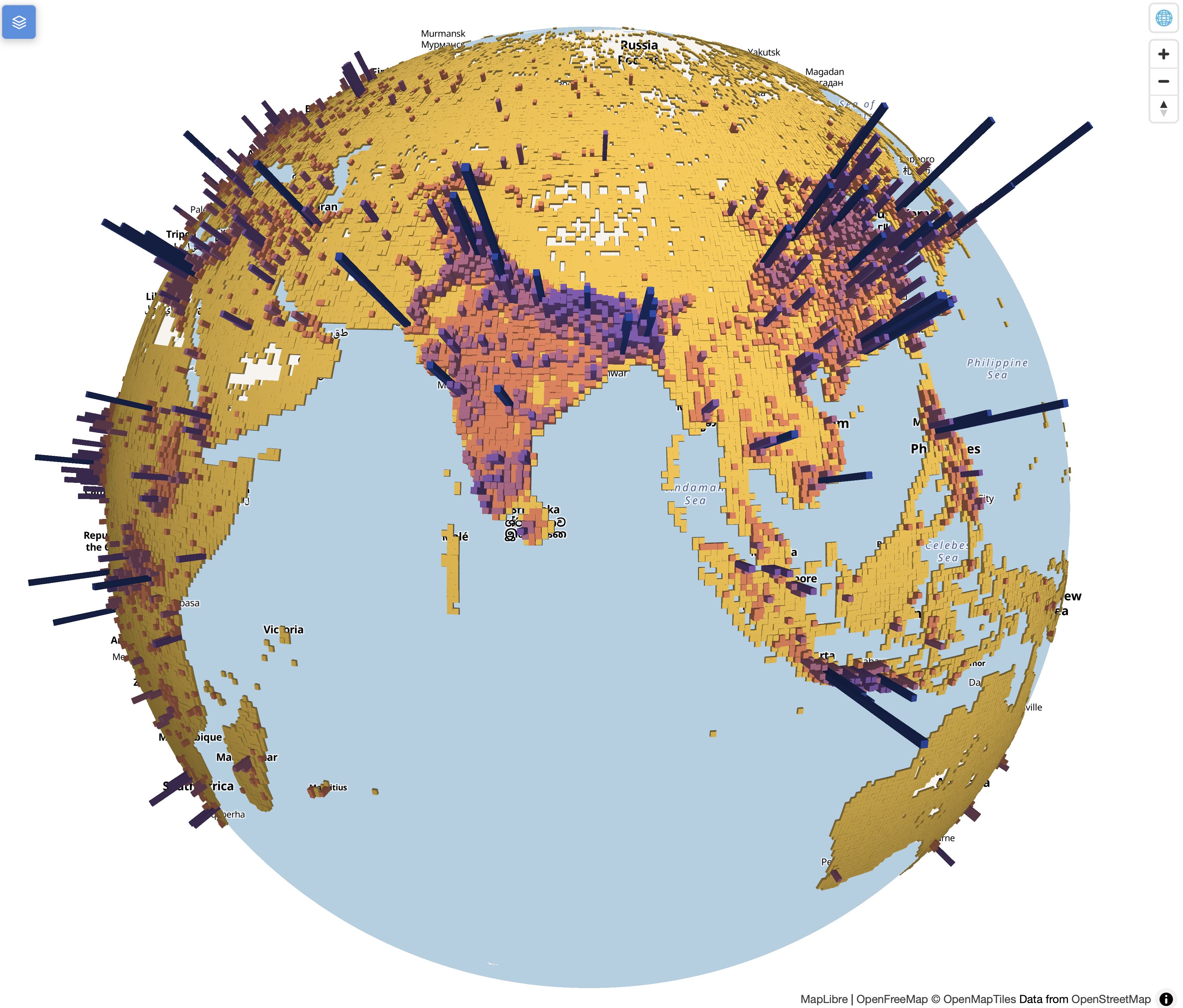
Global population density as extruded polygons. Height and colour both encode total population count.
Design notes for this map
- k-means intervals (
style = "kmeans") handle the highly skewed population distribution better than equal-interval or quantile "-ocean.thermal"— reversed sequential palette with good contrast across the range"ofm.bright"(OpenFreeMap) — a free, light basemap that contrasts well with the coloured barstm_legend_hide()— omitted because height already makes values readable spatially- Use
tmap_save(map, "map.html")to save as an interactive HTML file — the 3D map is fully interactive in the browser
High-performance mapping
Why performance matters
| Approach | Dataset size | Rendering | Notes |
|---|---|---|---|
Leaflet ("view") |
Small–medium | CPU | All data sent as GeoJSON |
| MapLibre/Mapbox | Medium–large | GPU (WebGL) | Much faster for large feature counts |
| Vector tiles | Very large | GPU (streaming) | Data loaded on demand per zoom level |
WebGL rendering
MapLibre and Mapbox GL render using WebGL — the GPU is involved:
- Smooth 60 fps zoom and pan
- Hundreds of thousands of features with minimal lag
- Especially useful for point clouds, dense line networks, and fine-grained polygon data
Leaflet re-renders in the DOM (Document Object Model — the browser’s internal representation of the page) on every interaction, using the CPU — slower at scale.
Memory constraints and the future
Current tmap processes all data in R memory before rendering.
Version 4.3 introduces initial support for PMTiles via tmap.sources (early development):
- PMTiles = a single-file archive format for vector/raster tiles served from remote storage
- Data is streamed to the browser without loading into R memory
- Scale functions (
tm_scale_intervals,tm_scale_categorical) generate browser-side rendering instructions instead of precomputing values in R
This makes truly large spatial datasets feasible in interactive tmap maps.
Emerging technologies
GeoArrow — compact columnar format for spatial data between R and the browser; avoids verbose GeoJSON. Together with WebGPU, enables much larger datasets.
Packages: geoarrowWidget, geoarrowDeckglLayers.
Direction of travel:
- Processing and rendering offloaded from R to the browser
- Both tmap and mapview are moving this way, with MapLibre as the primary backend (bridged to R via the mapgl package)
Practical guidance
✅ Use "view" (Leaflet) when:
- Quick interactive exploration
- Small to medium datasets (< ~10 000 features)
- Shiny apps where tmap integration is the priority
✅ Use "maplibre" when:
- Large datasets or many features
- Smooth UX is important for end users
- You need 3D visualisation
- You want high-quality map styles
Recap
tm_polygons_3d()adds aheightvisual variable for polygon extrusion- Camera tilt via
tm_maplibre(pitch = ...)(drag in browser to tilt interactively) - MapLibre/Mapbox use WebGL rendering — much faster than Leaflet at scale
- The WorldPop example shows how to combine
terra::aggregate()+tm_polygons_3d() - PMTiles + GeoArrow are the next frontier for large-data interactive mapping
- More: tmap.mapgl docs