tmap_mode("view")
tm_shape(your_data) +
tm_polygons(fill = "your_variable",
hover = "name",
popup.vars = c("name", "your_variable")) +
tm_basemap("CartoDB.Positron")Interactive Maps with tmap and Shiny
Session 12: Putting it all together: building a complete interactive map application
Martijn Tennekes
Course recap
What we covered
Day 1 — tmap foundations
- Session 1: Grammar, layer functions, naming conventions, version history
- Session 2: Interactive view mode — Leaflet, basemaps,
ttm() - Session 3: Legends and map components —
tm_legend(),tm_pos() - Session 4: Layer groups and controls —
group,group.control
Day 2 — Interactive maps
- Session 6: Tooltips and popups —
hover,popup.vars,id - Session 7: Introduction to tmap.mapgl — MapLibre, Mapbox,
rtm() - Session 8: 3D maps and high-performance —
tm_polygons_3d(), WebGL
Day 3 — Shiny
- Session 10: Export and sharing —
tmap_save(), HTML, animations - Session 11: tmap + Shiny —
renderTmap(),tmapProxy(), map events
The complete workflow
Data (sf, terra, stars)
    ↓
tmap specification (tm_shape + layers)
    ↓
Mode choice:
  "plot"     → static PNG/PDF via tmap_save()
  "view"     → interactive Leaflet HTML
  "maplibre" → interactive MapLibre GL HTML
    ↓
Output:
  Standalone HTML     → tmap_save(..., ".html")
  Shiny app           → renderTmap() + tmapProxy()
  Quarto / R Markdown → embed in code chunk
Case study: commuter flow explorer
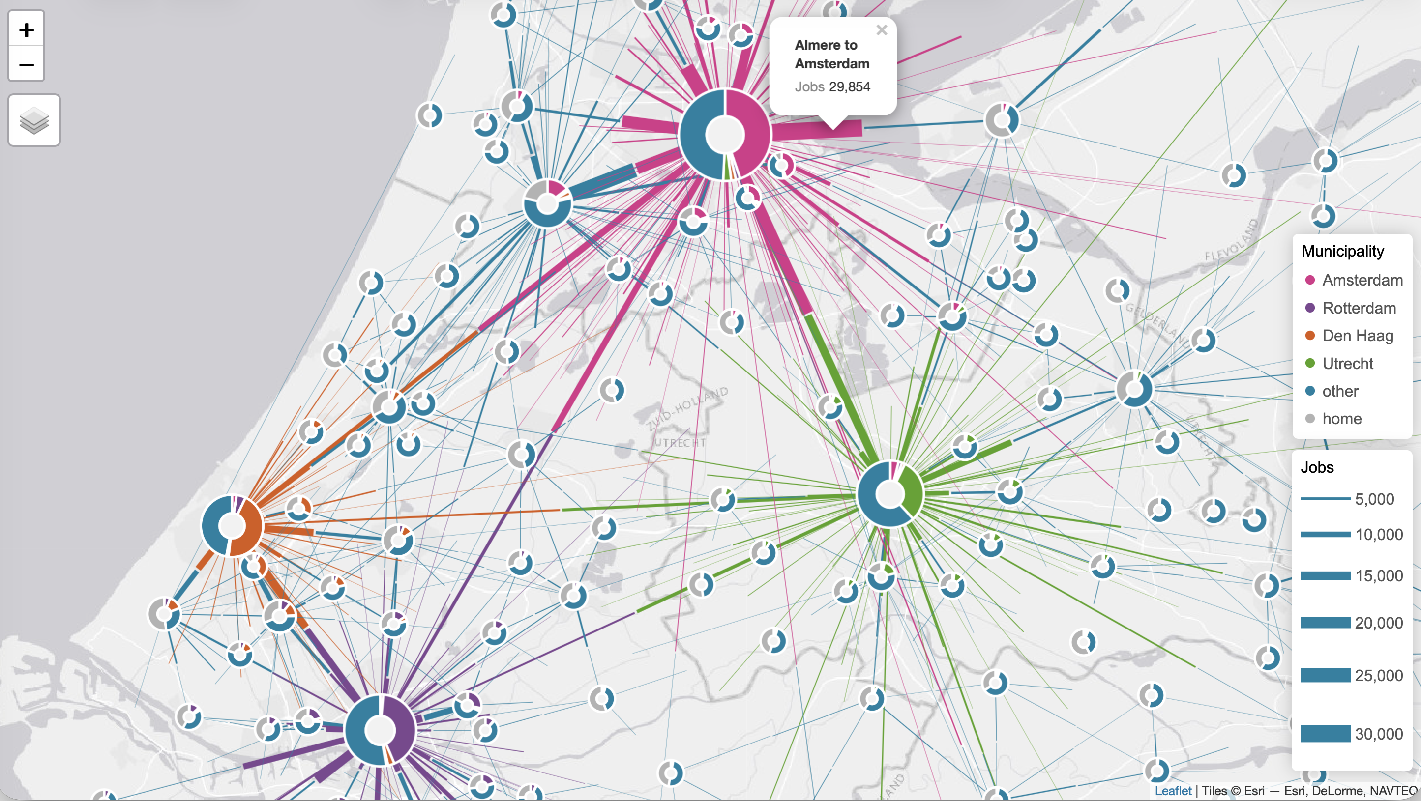
Donut maps
A donut map (Tennekes & Chen 2021) is a method for visualising origin-destination flows:
- Donut glyphs at each location: size = total volume; slices = share by origin
- Half-line edges: thickness = flow volume; colour = destination category
Built with tmap, tmap.networks, tmap.glyphs, and sfnetworks.
The map
How it is built
- OD flow data is prepared as an sfnetwork: municipality centroids as nodes, flows as directed edges
tm_edges()draws the half-lines —lwdencodes total flow,colencodes destination categorytm_donuts()places glyphs at each node —sizeencodes total jobs,partsencode the breakdown by origin- Layer groups (
"Flows","Donuts") let users toggle each layer independently hoverandpopup.varsmake both layers interactive
The Shiny app
A Shiny wrapper adds interactive controls:
- 4 city selectors — choose which municipalities are highlighted; reactive deduplication prevents selecting the same city twice
- Flow direction toggle — residents going to work vs workers coming in
- Sliders — minimum flow threshold and edge thickness range
- Update button — map only rebuilds on click (
eventReactive), avoiding expensive re-renders on every slider move - A
build_map()helper keeps the tmap logic separate from the Shiny boilerplate
Going further
What to explore next
More tmap features
- Facet maps (
tm_facets()) — small multiples - Animations (
tm_animate(),tmap_animation()) — time-lapse maps - Advanced legends —
tm_legend_combine(), bivariate legends tm_inset()— embed a zoomed-in detail or ggplot2 chart
tmap extensions
tmap.cartogram— contiguous, non-contiguous, and Dorling cartogramstmap.glyphs— donut and flower glyphs per featuretmap.networks— sfnetwork / igraph visualisation
Related packages
mapgl— direct access to Mapbox/MapLibrebslib— modern Shiny UI theming
Key resources
Hands-on assignment
Your turn
You have worked through three days of tmap. Now bring it all together with your own data.
The assignment has two parts:
- Build an interactive tmap map of your dataset
- Wrap it in a Shiny app with at least one control
Use the rest of this session to work on it — ask questions, explore, experiment.
Part 1: interactive map
Build an interactive tmap map of your own spatial data. Aim to include:
- At least one data layer with a meaningful variable (
fill,size, orcol) - Tooltips (
hover) and/or popups (popup.vars) - A basemap appropriate for your data
- Layer groups if you have more than one layer
Save it: tmap_save(m, "my_map.html")
Part 2: Shiny app
Wrap your map in a Shiny app with at least one input widget.
Suggested structure:
Ideas to extend
If you finish early, try adding one of these:
tmapProxy()— update only the fill variable without re-rendering the whole map- Click reaction — show details about a clicked feature in a
verbatimTextOutputortableOutput tm_minimap()— add a locator minimap- MapLibre mode — switch to
tmap_mode("maplibre")and see how the map changes (set beforeshinyApp()) - Export — add a
downloadButtonthat callstmap_save()to let users download the map as HTML
Recap — the whole course
- tmap offers a consistent, grammar-based API for both static and interactive maps
- Switching from
"plot"to"view"is often just one function call tmap.mapglunlocks GPU-accelerated rendering and 3D- Shiny integration makes tmap maps dynamic and user-driven
- The extension mechanism means tmap continues to grow without breaking existing code